Chapter 2. An Overview of x86 Architecture
2.1 Introduction
In our situation, and by using modern terminology, we can view the processor as a library and framework. A library because it provides us with a bunch of instructions to perform whatever we want, and a framework because it has general rules that organize the overall environment of execution, that is, it forces us to work in a specific way. We have seen some aspects of the first part when we have written the bootloader, that is, we have seen the processor as a library. In this chapter, we are going to see how the processor works as a framework by examining some important and basic concepts of x86. We need to understand these concepts to start the real work of writing 539kernel.
2.2 x86 Operating Modes
In x86 an operating mode specifies the overall picture of the processor, such as the maximum size of available registers, the available advanced features for the running operating system, the restrictions and so on.
When we developed the bootloader in the previous chapter we have worked with an x86 operating mode named real address mode (or for short real mode) which is an old operating mode that is still supported by modern x86 processors for the sake of backward compatibility, due to that when the computer is turned on, it initially runs on real mode.
Real mode is a 16-bit operating mode which means that, maximally, only 16 bits of register size can be used, even if the actual size of the registers is 64-bit. Using only 16 bits of registers has consequences other than the size itself, these consequences are considered as disadvantages in modern days, for example, in real mode the size of the main memory is limited, even if the computer has 16GB of memory, real mode can deal only with 1MB. Furthermore, any code which runs on real mode should be a 16-bit code, for example, the aforementioned 32-bit registers (such as eax) cannot be used in real mode code, their 16-bit counterparts should be used instead, as an example, the 16-bit ax should be used instead of eax and so on.
Some core features of modern operating systems nowadays are: multitasking, memory protection and virtual memory 1 and real mode provides nothing to implement these features. However, in modern x86 processors, new and more advanced operating modes have been introduced, namely, protected mode which is a 32-bit operating mode and long mode which is a relatively new 64-bit operating mode. Although the long mode provides more capacity for its users, for example, it can deal with 16 exabytes of memory, we are going to focus on protected mode since it provides the same basic mechanisms that we need to develop a modern operating system kernel with the aforementioned features, hence, 539kernel is a 32-bit kernel which runs under protected mode.
Since protected mode is a 32-bit operating mode then 32 bits of registers can be used, also, protected mode has the ability to deal with 4GB of main memory, and most importantly, it provides important features which we are going to explore through this book that helps us in implementing modern operating system kernel features.
As we have said before, multitasking is one of core features that modern operating systems provide. In multitasking environment more than one software can run at the same time, at least illusionary, even if there is only one processor or the current processor has only one core. For the sake of making our next discussion easier we should define the term process which means a program that is currently running. For example, if your web browser is currently running then this running instance of it is called a process, its code is loaded into the main memory and the processor is currently executing it. Another property of general-purpose operating systems is that they allow the user to run any software from unknown sources which means that these software cannot be trusted, they may contain code that intentionally or even unintentionally breach the security of the system or cause the system to crash.
Due to these two properties of modern general-purpose operating systems, the overall system needs to be protected from multiple actions. First, either in multitasking or monotasking 2 environment, the kernel of the operating system which is the most sensitive part of the system, should be protected from current processes, no process should be able to access any part of the kernel's memory either by reading from it or writing to it, also, no process should be able to call any of kernel's code without kernel's consent. Second, the sensitive instructions and registers that change the behavior of the processor (e.g. switching from real-mode to protected-mode) should be only allowed for the kernel which is the most privileged component of the system, otherwise, the stability of the system will be in danger. Third, in multitasking environment the running processes should be protected from each other in the same way the kernel is protected from them, no process should interfere with another.
In x86, the segmentation mechanism provided a logical view of memory in real-mode and it has been extended in protected-mode to provide the needed protection which has been described in the third point 3, while segmentation can be used in x86 for this kind of protection, it is not the sole way to perform that, the another well-known way is called paging, but segmentation is the default in x86 and cannot be turned off while paging is optional, the operating system has the option to use it as a way of memory protection or not.
Also, in the protected-mode the concept of privilege levels has been introduced to handle the protections needed in the previous first and second points. The academic literature of operating systems separate the system environment into two modes, kernel-mode and user-mode, at a given time, the system may run on one of these modes and not both of them. The kernel runs on kernel-mode, and has the privilege to do anything (e.g. access any memory location, access any resource of the system and perform any operation), while the user applications run on user-mode which is a restricted environment where the code that runs on doesn't have the privilege to perform sensitive actions.
This kind of separation has been realized through privilege levels in x86 which provides four privilege levels numbered from 0 to 3. The privilege level 0 is the most privileged level which can be used to realize the kernel-mode while the privilege level 3 is the least privileged which can be used to realize the user-mode. For privilege levels 1 and 2 it's up to the kernel's designer to use them or not, some kernel designs suggest to use these levels for device drivers. According to Intel's manual, if the kernel's design uses only two privilege levels, that is, a kernel-mode and user-mode, then the privilege level 0 and 3 should be used and not for example 0 and 1.
In addition to protecting the kernel's code from being called without its consent and protecting kernel's data from being accessed by user processes (as both required by first point above), the privilege levels also prevent user processes 4 from executing privileged instructions (as required by second point above), only the code which runs in the privilege level 0, that is, the kernel, will be able to execute these instructions since they could manipulate sensitive parts of the processor's environment 5 that only the kernel should maintain.
When a system uses different privilege levels to run, as in most modern operating systems, the x86 processor maintains what is called current privilege level (CPL) which is, as its name suggests, the current privilege level of the currently running code. For example, if the currently running code belongs to the kernel then the current privilege level will be 0 and according to it, the processor is going to decide allowed operations. In other words, we can say that the processor keeps tracking the current state of the currently running system and one of the information in this state is in which privilege level (or mode) the system is currently running.
2.3 Numbering Systems
The processor works with all values as binary numbers while it is natural for us as human beings to deal with numbers as decimal numbers. A number by itself is an abstract concept, it is something in our mind, but to communicate with each others, we represent the numbers by using symbols which is named numerals. For example, the conceptual number one can be represented by different numeral systems. In Arabic numeral system the number one is expressed as 1, while in Roman numeral system it is expressed as I.
A numeral system is writing system, that is, it gives us rules of how to write a number down as a symbol, it focuses on the way of writing the numbers. On the other hand, the numbers can be dealt with by a numbering system, we use the decimal numbering system to deal with numbers, think about them and perform arithmetic operations upon them, the processor uses the binary numbering system to do the same with numbers. There are numbering systems other than the decimal and binary numbering system, and any number can be represented by any numbering system.
A number system is defined by its base which is also called radix, this base defines the list of available digits in the numbering system starting from 0 to base - 1, the total of available digits equals the base. Consider the decimal numbering system, its base is 10 which means the available digits in this system are: 0, 1, 2, 3, 4, 5, 6, 7, 8, 9, a total of 10 digits. These digits can be used to create larger numbers, for example, 539 which consists of the digits 5, 3 and 9.
On the other hand, the base of binary numbering system is 2, therefore, the available digits are only 0 and 1, and as in the decimal numbering system they can be used to compose larger numbers, for example, the number two in binary numbering system is 10 6, be careful, this numeral does not represent the number ten, it represents the number two but in binary numbering system. When we discuss numbers in different numbering systems, we put the initial letter of the numbering system name in the end of the number, for example, 10d and 10b are two different numbers, the first one is ten in decimal while the second one is two in binary.
Furthermore, basic arithmetic operations such as addition and subtraction can be performed on the numbering system, for example, in binary 1 + 1 = 10 and it can be performed systematically, also, a representation of any number in any numbering system can be converted to any other numbering system systematically 7, while this is not a good place to show how to perform the operations and conversions for different numbering system, you can find many online resources that explain these operations on the well-known number systems.
By now it should be obvious for you that changing the base (radix) gives us a new numbering system and the base can be any number which implies that the total of numbering systems is infinite! One of useful and well-known numbering system is hexadecimal which its base is 16 and its digits are 0, 1, 2, 3, 4, 5, 6, 7, 8, 9, A, B, C, D, E, F where A means ten, B means eleven and so on. So, why hexadecimal is useful in our situation? Since binary is used in the processor it will be easier to discuss some related entities such as the value of FLAGS register which each bit on it represents a value for a different thing, another example is memory addresses. But consider the following example which is a binary number that represents a memory address.
00000000 00000000 00000000 00000001bIt is too long and it will be tedious to work with, and for that the hexadecimal numbering system can be useful. Each digit in hexadecimal represents four bits 8, that is, the number 0h in hexadecimal is equivalent to 0000b in binary. As the 8 bits known as a byte, the 4 bits is known as a nibble, that is, a nibble is a half byte and, as we have said, but in other words, one digit of hexadecimal represents a nibble. So, we can use hexadecimal to represent the same memory address value in more elegant way.
00 00 00 01h| Decimal | Binary | Hexadecimal |
|---|---|---|
| 0 | 0 | 0 |
| 1 | 1 | 1 |
| 2 | 10 | 2 |
| 3 | 11 | 3 |
| 4 | 100 | 4 |
| 5 | 101 | 5 |
| 6 | 110 | 6 |
| 7 | 111 | 7 |
| 8 | 1000 | 8 |
| 9 | 1001 | 9 |
| 10 | 1010 | A |
| 11 | 1011 | B |
| 12 | 1100 | C |
| 13 | 1101 | D |
| 14 | 1110 | E |
| 15 | 1111 | F |
2.4 The Basic View of Memory
The basic view of the main memory is that it is an array of cells, each cell has the ability to store one byte and it is reachable by a unique number called memory address 9, the range of memory addresses starts from 0 to some limit x, for example, if the system has 1MB of physical main memory, then the last memory address in the range will be 1023, as we know, 1MB = 1024 bytes and since the range starts from 0 and not 1, then the last memory address in this case is 1023 and not 1024. This range of memory addresses is known as address space and it can be a physical address space which is limited by the physical main memory or a logical address space. A well-known example of using logical address space that we will discuss in a latter chapter is virtual memory which provides a logical address space of size 4GB in 32-bit architecture even if the actual size of physical main memory is less than 4GB. However, The address space starts from the memory address 0, which is the index of the first cell (byte) of the memory, and it increases by 1, so the memory address 1 is the index of the second cell of the memory, 2 is the index of third cell of memory and so on. Viewing the memory as an array of contiguous cells is also known as flat memory model.

Figure 1: The Physical View of the Memory. The Size of it is n Bytes.
When we say physical we mean the actual hardware, that is, when the maximum capacity of the hardware of the main memory (RAM) is 1MB then the physical address space of the machine is up to 1MB. On the other hand, when we say logical that means it doesn't necessarily represents or obeys the way the actual hardware works on, instead it is a hypothetical way of something that doesn't exist in the real world (the hardware). To make the logical view of anything works, it should be mapped into the real physical view, that is, it should be somehow translated for the physical hardware to be understood, this mapping is handled by the software or sometimes special parts of the hardware.
Now, for the following discussion, let me remind you that the memory address is just a numerical value, it is just a number. When I discuss the memory address as a mere number I call it memory address value or the value of memory address, while the term memory address keeps its meaning, which is a unique identifier that refers to a specific location (cell) in the main memory.
The values of memory addresses are used by the processor all the time to be able to perform its job, and when it is executing some instructions that involve the main memory (e.g. reading a content from some memory location or dealing with program counter), the related values of memory addresses are stored temporarily on the registers of the processor, due to that, the length of a memory address value is bounded to the size of the processor's registers, so, in 32-bit environments, where the size of the registers is usually 32-bit, the length of the memory address value is always 32 bits, why am I stressing "always" here? Because even if less than 32 bits is enough to represent the memory address value, it will be represented in 32 bits though, for example, assume the memory address value 1, in binary, the value 1 can be represented by only 1 bit and no more, but in reality, when it is stored (and handled) by the 32-bit processor, it will be stored as the following sequence of bits.
00000000 00000000 00000000 00000001As you can see, the value 1 has been represented in exactly 32 bits, appending zeros to the left doesn't change the value itself, it is similar to writing a number as 0000539 which is exactly 539.
It has been mentioned earlier that the register size that stores the values of memory address in order to deal with memory contents affects the available size of main memory for the system. Take for example the instruction pointer register, if its size, say, 16 bits then the maximum available memory for code will be 64KB (64 KB = 65536 Bytes / 1024) since it is the last reachable memory address by the processor for fetching an instruction. What if the size of the instruction pointer register is 32 bits, then the maximum available memory for code will be 4GB. Why is that?
To answer this question let's work with decimal numbers first. If I tell you that you have five blanks, what is the largest decimal number you can represent in these five blanks? the answer is 99999d. In the same manner, if you have 5 blanks, what is the largest binary number you can represent in these 5 blanks? it is 11111b which is equivalent to 31d, the same holds true for the registers that store the value of memory addresses, given the size of such register is 16 bits, then there is 16 blanks, and the largest binary number that can be represented in those 16 blanks is 11111111 11111111b or in hexadecimal FF FFh, which is equivalent to 65535d, that means the last byte a register of size 16 bits can refer to is the byte number 65535d because it is the largest value this register can store and no more, which leads to the maximum size of main memory this register can handle, it is 65535 bytes which is equivalent to 64KB and the same applies on any other size than 16 bits.
2.5 x86 Segmentation
The aforementioned view of memory, that is, the addressable array of bytes can be considered as the physical view of the main memory which specifies the mechanism of accessing the data. On top of this physical view a logical view can be created and one example of logical views is x86 segmentation.
In x86 segmentation the main memory is viewed as separated parts called segments and each segment stores a bunch of related data. To access data inside a segment, each byte can be referred to by its own offset. The running program can be separated into three possible types of segments in x86, these types are: code segment which stores the code of the program under execution, data segments which store the data of the program and the stack segment which stores the data of program's stack. Segmentation is the default view of memory in x86 and it's unavoidable and the processor always run with the mind that the running program is divided into segments, however, most modern operating system choose to view the memory as the one described in flat memory model instead of viewing it as segmented areas, to be able to implement flat memory model in x86 which doesn't allow to disable segmentation, at least two segments (one for code and one for data) should be defined in the system, and the size of both segments should be same as physical memory's size and both of segments start from the first memory address 0 and ends in the last memory address (memory size - 1), that is, these both segments will overlap.

Figure 2: An Example of The Segmented View of the Memory
2.5.1 Segmentation in Real Mode
For the sake of clarity, let's discuss the details of segmentation under real mode first. We have said that logical views (of anything) should be mapped to the physical view either by software or hardware, in this case, the segmentation view is realized and mapped to the architecture of the physical main memory by the x86 processor itself, that is, by the hardware. So, we have a logical view, which is the concept of segmentation which divides a program into separated segments, and the actual physical main memory view which is supported by the real RAM hardware and sees the data as a big array of bytes. Therefore, we need some tools to implement (map) the logical view of segmentation on top the actual hardware.
For this purpose, special registers named segment registers are presented in x86, the size of each segment register is 16 bits and they are: CS which is used to define the code segment. SS which is used to define the stack segment. DS, ES, FS and GS which can be used to define data segments, that means each program can have up to four data segments. Each segment register stores the starting memory address of a segment and here you can start to observe the mapping between the logical and physical view. In real mode, the size of each segment is 64KB and as we have said we can reach any byte inside a segment by using the offset of the required byte, you can see the resemblance between a memory address of the basic view of memory and an offset of the segmentation view of memory 10.
Let's take an example to make the matter clear, assume that we have a code of some program loaded into the memory and its starting physical memory address is 100d, that is, the first instruction of this program is stored in this address and the next instructions are stored right after this memory address one after another. To reach the first byte of this code we use the offset 0, so, the whole physical address of the first byte will be 100:0d, as you can see, the part before the colon is the starting memory address of the code and the part after the colon is the offset that we would like to reach and read the byte inside it. In the same way, let's assume we would like to reach the offset 33, which means the byte 34 inside the loaded code, then the physical address that we are trying to reach is actually 100:33d. To make the processor handle this piece of code as the current code segment then its starting memory address should be loaded into the register CS, that is, setting the value 100d to CS, so, we can say in other words that CS contains the starting memory address of currently executing code segment (for short: current code segment).
As we have said, the x86 processor always run with the mind that the segmentation is in use. So, let's say it is executing the following assembly instruction jmp 150d which jumps to the address 150d. What really happens here is that the processor consider the value 150d as an offset instead of a full memory address, so, what the instruction requests from the processor here is to jump to the offset 150 which is inside the current code segment, therefore, the processor is going to retrieve the value of the register CS to know what is the starting memory address of the currently active code segment and append the value 150 to it. Say, the value of CS is 100, then the memory address that the processor is going to jump to is 100:150d.
This is also applicable on the internal work of the processor, do you remember the register IP which is the instruction pointer? It actually stores the offset of the next instruction instead of the whole memory address of the instruction. Any call (or jump) to a code inside the same code segment of the caller is known as near call (or jump), otherwise is it a far call (or jump). Again, let's assume the current value of CS is 100d and you want to call a label which is on the memory location 900:1d, in this situation you are calling a code that reside in a different code segment, therefore, the processor is going to take the first part of the address which is900d, loads it to CS then loads the offset 1d in IP. Because this call caused the change of CS value to another value, it is a far call.
The same is exactly applicable to the other two types of segments and of course, the instructions deal with different segment types based on their functionality, for example, you have seen that jmp and call deal the code segment in CS, that's because of their functionality which is related to the code. Another example is the instruction lodsb which deals with the data segment DS, the instruction push deals with the stack segment SS and so on.
2.5.1.1 Segmentation Used in the Bootloader
In the previous chapter, when we wrote the bootloader, we have dealt with the segments. Let's get back to the source code of the bootloader, you remember that the firmware loads the bootloader on the memory location 07C0h and because of that we started our bootloader with the following lines.
    mov ax, 07C0h
    mov ds, ax
Here, we told the processor that the data segment of our program (the bootloader) starts in the memory address 07C0h 11, so, if we refer to the memory to read or write data, the processor starts with the memory address 07C0h which is stored in the data segment register ds and then it appends the offset that we are referring to, in other words, any reference to data by the code being executed will make the processor to use the value in data segment register as the beginning of the data segment and the offset of referred data as the rest of the address, after that, this physical memory address of the referred data will be used to perform the instruction. An example of instructions that deal with data in our bootloader is the line mov si, title_string.
Now assume that BIOS has set the value of ds to 0 (it can be any other value) and jumped to our bootloader, that means the data segment in the system now starts from the physical memory address 0 and ends at the physical memory address 65535 since the maximum size of a segment in real-mode is 64KB. Now let's take the label title_string as an example and let's assume that its offset in the binary file of our bootloader is 490, when the processor starts to execute the line mov si, title_string 12 it will, somehow, figures that the offset of title_string is 490 and based on the way that x86 handles memory accesses the processor is going to think that we are referring to the physical memory address 490 since the value of ds is 0, but in reality, the correct physical memory address of title_string is the offset 490 inside the memory address 07C0h since our bootloader is loaded into this address and not the physical memory address 0, so, to be able to reach to the correct addresses of the data that we have defined in our bootloader and that are loaded with the bootloader starting from the memory address 07C0h we need to tell the processor that our data segment starts from 07C0h and with any reference to data, it should calculate the offset of that data starting from this physical address, and that exactly what these two lines do, in other words, change the current data segment to another one which starts from the first place of our bootloader.
The second use of the segments in the bootloader is when we tried to load the kernel from the disk by using the BIOS service 13h:02h in the following code.
    mov ax, 0900h
    mov es, ax

    mov ah, 02h
    mov al, 01h
    mov ch, 0h
    mov cl, 02h
    mov dh, 0h
    mov dl, 80h
    mov bx, 0h
    int 13h
You can see here, we have used the other data segment ES to define a new data segment that starts from the memory address 0900h, we did that because the BIOS service 13h:02h loads the required content (in our case the kernel) to the memory address ES:BX, for that, we have defined the new data segment and set the value of bx to 0h. That means the code of the kernel will be loaded on 0900:0000h and because of that, after loading the kernel successfully we have performed a far jump.
jmp 0900h:0000Once this instruction is executed, the value of CS will be changed from the value 07C0h, where the bootloader resides, to the value 0900h where the kernel resides and the value of IP register will be 0000 then the execution of the kernel is going to start.
2.5.2 Segmentation in Protected Mode
The fundamentals of segmentation in protected mode is exactly same as the ones explained in real mode, but it has been extended to provide more features such as memory protection. In protected mode, a table named global descriptor table (GDT) is presented, this table is stored in the main memory and its starting memory address is stored in the special purpose register GDTR as a reference, each entry in this table called a segment descriptor which has the size 8 bytes and they can be referred to by an index number called segment selector 13 which is the offset of the entry inside GDT table, For example, the offset of the first entry in GDT is 0, and adding this offset with the value of GDTR gives us the memory address of that entry, however, the first entry of GDT should not be used by the operating system.
An entry of GDT (a segment descriptor), defines a segment (of any type) and has the information that is required by the processor to deal with that segment. The starting memory address of the segment is stored in its descriptor 14, also, the size (or limit) of the segment. The segment selector of the currently active segment should be stored in the corresponding segment register.
To clarify the matter, consider the following example. Let's assume we are currently running two programs and their code are loaded into the main memory and we would like to separate these two pieces of code into a couple of code segments. The memory area A contains code of the first program and starts from the memory address 800 while the memory area B contains the code of the second programB and starts in the memory address 900. Assume that the starting memory address of GDT is 500 which is already loaded in GDTR.
To make the processor consider A and B as code segments we should define a segment descriptor for each one of them. We already know that the size of a segment descriptor is 8 bytes, so, if we define a segment descriptor for the segment A as entry 1 (remember that the entries on GDT starts from zero) then its offset (segment selector) in GDT will be 8 (1 * 8), the segment descriptor of A should contain the starting address of A which is 800, and we will define the segment descriptor of B as entry 2 which means its offset (segment selector) will be 16 (2 * 8).
Let's assume now that we want the processor to execute the code of segment A, we already know that the processor consults the register CS to decide which code segment is currently active and should be executed next, for that, the segment selector of code segment A should be loaded in CS, so the processor can start executing it. In real mode, the value of CS and all other segment registers was a memory address, on the other hand, in protected mode, the value of CS and all other segment registers is a segment selector.
In our situation, the processor takes the segment selector of A from CS which is 8 and starting from the memory address which is stored in GDTR it walks 8 bytes, so, if GDTR = 500, the processor will find the segment descriptor of A in the memory address 508. The starting address of A will be found in its segment descriptor and the processor can use it with the value of register EIP to execute A's code. Let's assume a far jump is occurred from A to B, then the value of CS will be changed to the segment selector of B which is 16.
2.5.2.1 The Structure of Segment Descriptor
A segment descriptor is an 8 bytes entry of global descriptor table which stores multiple fields and flags that describe the properties of a specific segment in the memory. With each memory reference to any segment, the processor is going to consult the descriptor that describes the segment in question to obtain basic information like starting memory address of this segment.
Beside the basic information, a segment descriptor stores information the helps in memory protection, due to that, segmentation in x86 protected-mode is considered as a way for memory protection and not a mere logical view of the memory, so each memory reference is being monitored by the processor.
By using those properties that are related to memory protection, the processor will be able to protect the different segments on the system from each other and not letting some less privileged to call a code or manipulate data which belong to more privileged area of the system, a concrete example of that is when a userspace software (e.g. Web Browser) tries to modify an internal data structure in the kernel.
In the following subsections, each field and flag of segment descriptor will be explained, but before getting started we need to note that in here and in Intel's official x86 manual the term field is used when the size of the value that should be stored in the descriptor is more than 1 bit, for example the segment's starting memory address is stored in 4 bytes, then the place where this address is stored in the descriptor is called a field, otherwise when the term flag is used that means the size of the value is 1 bit.
2.5.2.1.1 Segment's Base Address and Limit
The most important information about a segment is its starting memory address, which is called the base address of a segment. In real mode, the base address was stored in the corresponding segment register directly, but in protected mode, where we have more information about a segment than mere base address, this information is stored in the descriptor of the segment 15.
When the currently running code refers to a memory address to read from it, write to it (in the case of data segments) or call it (in the case of code segments) it is actually referring to a specific segment in the system 16. For the simplicity of next discussions, we call this memory address, which is referenced by the currently running code, the generated memory address because, you know, it is generated by the code.
Any generated memory address in x86 architecture is not an actual physical memory address 17, that means, if you hypothetically get a generated memory address and try to get the content of its physical memory location, the obtained data will not be same as the data which is required by the code. Instead, a generated memory address is named by Intel's official manual a logical memory address because, you know, it is not real memory address, it is logical. Every logical memory address refers to some byte in a specific segment in the system, and to be able to obtain the data from the actual physical memory, this logical memory address should be translated to a physical memory address 18.
The logical memory address in x86 may pass two translation processes instead of one in order to obtain the physical memory address. The first address translation is performed on a logical memory address to obtain a linear memory address which is another not real and not physical memory address which is there in x86 architecture because of paging feature. If paging 19 is enabled in the system, a second translation process takes place on this linear memory address to obtain the real physical memory address. If paging is disabled, the linear memory address which is generated by the first translation process is same as the physical memory address. We can say that the first translation is there in x86 due to the segmentation view of memory, while the second translation is there in x86 due to the paging view of memory.

Figure 3: Shows How a Logical Memory Address is Translated to a Linear Memory Address (Which Represents a Physical Address when Paging is Disabled).
For now, our focus will be on the translation from a logical memory address to a linear memory address which is same as the physical memory address since paging feature is disabled by default in x86. Each logical memory address consists of two parts, a 16 bits segment selector and a 32 bits offset. When the currently running code generates a logical memory address (for instance, to read some data from memory) the processor needs to perform the translation process to obtain the physical memory address as the following. First, it reads the value of the register GDTR which contains the starting physical memory address of GDT, then it uses the 16-bit segment selector in the generated logical address to locate the descriptor of the segment that the code would like to read the data from, inside segment's descriptor, the physical base address (the starting physical address) of the requested segment can be found, the processor obtains this base address and adds the 32-bit offset from the logical memory address to the base address to obtain the last result, which is the linear memory address.
During this operation, the processor uses the other information in the segment descriptor to enforce the policies of memory protection. One of these policies is defined by the limit of a segment which specifies its size, if the generated code refers to an offset which exceeds the limit of the segment, the processor should stop this operation. For example, assume hypothetically that the running code has the privilege to read data from data segment A and in the physical memory another data segment B is defined right after the limit of A, which means if we can exceed the limit of A we will able to access the data inside B which is a critical data segment that stores kernel's internal data structures and we don't want any code to read from it or write to it in case this code is not privileged to do so. This can be achieved by specifying the limit of A correctly, and when the unprivileged code tries maliciously to read from B by generating a logical memory address that has an offset which exceeds the limit of A the processor prevents the operation and protects the content of segment B.
The limit, or in other words, the size of a given segment is stored in the 20 bits segment limit field of that segment descriptor and how the processor interprets the value of segment limit field depends on the granularity flag (G flag) which is also stored in the segment's descriptor, when the value of this flag is 0 then the value of the limit field is interpreted as bytes, let's assume that the limit of a given segment is 10 and the value of granularity flag is 0, that means the size of this segment is 10 bytes. On the other hand, when the value of granularity flag is 1, the value of segment limit field will be interpreted as of 4KB units, for example, assume in this case that the value of limit field is also 10 but G flag = 1, that means the size of the segment will be 10 of 4KB units, that is, 10 * 4KB which gives us 40KB which equals 40960 bytes.
Because the size of segment limit field is 20 bits, that means the maximum numeric value it can represent is 2^20 = 1,048,576, which means if G flag equals 0 then the maximum size of a specific segment can be 1,048,576 bytes which equals 1MB, and if G flag equals 1 then the maximum size of a specific segment can be 1,048,576 of 4KB units which equals 4 GB.
Getting back to the structure of descriptor, the bytes 2, 3 and 4 of the descriptor store the least significant bytes of segment's base address and the byte 7 of the descriptor stores the most significant byte of the base address, the total is 32 bits for the base address. The bytes 0 and 1 of the descriptor store the least significant bytes of segment's limit and byte 6 stores the most significant byte of the limit. The granularity flag is stored in the most significant bit of the the byte 6 of the descriptor.
Before finishing this subsection, we need to define the meaning of least significant and most significant byte or bit. Take for example the following binary sequence which may represent anything, from a memory address value to a UTF-32 character.
0111 0101 0000 0000 0000 0000 0100 1101
You can see the first bit from left is on bold format and its value is 0, based on its position in the sequence we call this bit the most significant bit or high-order bit, while the last bit on the right which is in italic format and its value is 1 is known as least significant bit or low-order bit. The same terms can be used on byte level, given the same sequence with different formatting.
0111 0101 0000 0000 0000 0000 0100 1101
The first byte (8 bits) on the left which is in bold format and its value is 0111 0101 is known as most significant byte or high-order byte while the last byte on the right which is on italic format and its value is 0100 1101 is known as least significant byte or low-order byte.
Now, imagine that this binary sequence is the base address of a segment, then the least significant 3 bytes of it will be stored in bytes 2, 3 and 4 of the descriptor, that is, the following binary sequence.
0000 0000 0000 0000 0100 1101While the most significant byte of the binary sequence will be stored in the 7th byte of the descriptor, that is, the following binary sequence.
0111 01012.5.2.1.2 Segment's Type
Given any binary sequence, it doesn't have any meaning until some context is added. For example, what does the binary sequence 1100 1111 0000 1010 represents? It could represent anything, a number, characters, pixels on an image or even all of them based on how its user interprets it. When an agent (e.g. a bunch of code in running software or the processor) works with a binary sequence, it should know what does this binary sequence represent to be able to perform useful tasks. In the same manner, when a segment is defined, the processor (the agent) should be told how to interpret the content inside this segment, that is, the type of the segment should be known by the processor.
Till this point, you probably noticed that there is at least two types of segments, code segment and data segment. The content of the former should be machine code that can be executed by the processor to perform some tasks, while the content of the latter should be data (e.g. values of constants) that can be used by a running code. These two types of segments (code and data) belong to the category of application segments, there is another category of segment types which is the category of system segments and it has many different segment types belong to it.
Whether a specific segment is an application or system segment, this should be mentioned in the descriptor of the segment in a flag called S flag or descriptor type flag which is the fifth bit in byte number 5 of the segment descriptor. When the value of S flag is 0, then the segment is considered as a system segment, while it is considered as an application segment when the value of S flag is 1. Our current focus is on the latter case.
As we have mentioned before, an application segment can be either code or data segment. Let's assume some application segment has been referenced by a currently running code, the processor is going to consult the descriptor of this segment, and by reading the value of S flag (which should be 1) it will know that the segment in question is an application segment, but which of the two types? Is it a code segment or data segment? To answer this question for the processor, this information should be stored in a field called type field in the segment's descriptor.
Type field in segment descriptor is the first 4 bits (nibble) of the fifth byte and the most significant bit specifies if the application segment is a code segment (when the value of the bit is 1) or a data segment (when the value of the bit is 0). Doesn't matter if the segment is a code or data segment, in the both cases the least significant bit of type field indicates if the segment is accessed or not, when the value of this flag is 1, that means the segment has been written to or read from (AKA: accessed), but if the value of this flag is 0, that means the segment has not been accessed. The value of this flag is manipulated by the processor in one situation only, and that's happen when the selector of the segment in question is loaded into a segment register. In any other situation, it is up to the operating system to decide the value of accessed flag. According to Intel's manual, this flag can be used for virtual memory management and for debugging.
2.5.2.1.2.1 Code Segment Flags
When the segment is a code segment, the second most significant bit (tenth bit) is called conforming flag (also called C flag) while the third most significant bit (ninth bit) called read-enabled flag (also called R flag.). Let's start our discussion with the simplest among those two flags which is the read-enabled flag. The value of this flag indicates how the code inside the segment in question can be used, when the value of read-enabled flag is 1 20, that means the content of the code segment can be executed and read from, but when the value of this flag is 0 21 that means the content of the code segment can be only executed and cannot read from. The former option can be useful when the code contains data inside it (e.g. constants) and we would like to provide the ability of reading this data. When read is enabled for the segment in question, the selector of this segment can also be loaded into one of data segment registers 22.
The conforming flag is related to the privilege levels that we had an overview about them previously in this chapter. When a segment is conforming, in other words, the value of conforming flag is 1, that means a code which runs in a less-privileged level can call this segment which runs in a higher privileged level while keeping the current privilege level of the environment same as the one of the caller instead of the callee.
For example, let's assume for some reason a kernel's designer decided to provide simple arithmetic operations (such as addition and subtraction) for user applications from the kernel code, that is, there is no other way to perform these operations in that system but this code which is provided by the kernel. As we know, kernel's code should run in privilege level 0 which is the most-privileged level, and let's assume a user application which runs in privilege level 3, a less-privileged level, needs to perform an addition operation, in this case a kernel code, which should be protected by default from being called by less-privileged code, should be called to perform the task, this can only realized if the code of addition operation is provided as a conforming segment, otherwise the processor is going to stop this action where a less-privileged code calls a more-privileged code.
Also you should note that the code of addition operation is going to run in privilege level 3 although it is a part of the kernel which runs in privilege level 0 and that's because of the original caller which runs in the privilege level 3. Furthermore, although conforming segment can be called by a less-privilege code (e.g. user application calls the kernel), the opposite cannot be done (e.g. the kernel calls a user application's code) and the processor is going to stop the operation.
2.5.2.1.2.2 Data Segment Flags
When the segment is data segment, the second most significant bit (tenth bit) is called expansion-direction flag (also called E flag) while the third most significant bit (ninth bit) is called write-enabled flag (also called W flag). The latter one gives us the ability to make some data segment a read-only when its value is 0, or we can make a data segment both writable and readable by setting the value of write-enabled flag to 1.
While the expansion-direction flag and its need will be examined in details when we discuss x86 run-time stack in this chapter, what we need to know right now is that when the value of this flag is 0, the data segment is going to expand up (in Intel's terms), but when the value of this flag is 1, the data segment is going to expand down (in Intel's terms).
A last note about data segments is that all of them are non-conforming, that is, a less-privileged code cannot access a data segment in a more-privileged level. Furthermore, all data segments can be accessed by a more-privileged code.
2.5.2.1.3 Segment's Privilege Level
In our previous discussions, we have stated that a specific segment should belong to a privilege level and based on this privilege level the processor decides the protection properties of the segment in question, for example, whether that segment is a kernel-mode or user-mode segment and which privilege level a running code should belong to in order to be able to reach to this segment
A field called descriptor privilege level (DPL) in segment descriptor is where the operating system should set the privilege level of a given segment. The possible values of this field, as we know, are 0, 1, 2 and 3, we have already discussed the meanings of these values previously in this chapter. Descriptor privilege level field occupies the second and third most significant bits of byte 5 in a descriptor.
2.5.2.1.4 Segment's Present
One of common operations that is performed in a running system is loading data from secondary storage (e.g. hard disk) into the memory and one example of that is loading a program code into the memory when the user of the system request to run an instance of a program, so, creating a new segment descriptor (hence, creating new segment in the memory) for this data may precede the completion of loading the data into the main memory, therefore, there could be some segment descriptors in the system that points to memory locations that don't contain the real data yet.
In this case, we should tell the processor that the data in the memory location that a specific descriptor points to is not the real data, and the real segment is not presented in the memory yet, this helps the processor to generate error when some code tries to access 23 the segment's data. To tell the processor whether a segment is presented in the memory or not, segment-present flag (P flag) can be used, when its value is 1 that means the segment is present in memory, while the value 0 means the segment is not present in memory, this flag is the most significant bit of byte 5 of a descriptor.
2.5.2.1.5 Other Flags
We have covered all segment's descriptor fields and flags but three flags. The name of the first one changes depending on the type of the segment and it occupies the second most significant bit in the byte 6. When the segment in question is a code segment, this flag is called default operation size (D flag). When the processor executes the instructions it uses this flag to decide the length of the operands, depending on the currently executing instruction, if the value of D flag is 1 the processor is going to assume the operand has the size of 32 bits if it is a memory address, and 32 bits or 8 bits if it is not a memory address. If the value of D flag is 0 the processor is going to assume the operand has the size of 16 bits if it is a memory address, and 16 bits or 8 bits operand if it is not a memory address.
When the segment in question is a stack segment 24, the same flag is called default stack pointer size (B flag), and it decides the size of the memory address (as a value) which points to the stack, this memory address is known as stack pointer and it is being used implicitly by stack instructions such as push and pop. When the value of B flag is 1, then the size of stack pointer will be 32 bits and its value will be stored in the register ESP (rather then SP), When the value of B flag is 0, then the size of stack pointer will be 16 bits and its value will be stored in the register SP (rather then ESP).
When the segment in question is a data segment that grows upward, this flag is called upper bound flag (B flag), when its value is 1 the maximum possible size of the segment will be 4GB, otherwise, the maximum possible size of the segment will be 64KB. Anyway, the value of this flag (D/B flag) should be 1 for 32-bit code and data segments (stack segments are included of course) and it should be 0 for 16-bit code and data segments.
The second flag is known as 64-bit code segment flag (L flag) which is the third most significant bit in the byte 6 and from its name we can tell that this flag is related to code segments. If the value of this flag is 1 that means the code inside the segment in question is a 64-bit code while the value 0 means otherwise 25. When we set the value of L flag to 1 the value of D/B flag should be 0.
The final flag is the fourth most significant bit in the byte 6, the value of this flag has no meaning for the processor, hence, it will not use it to make any decisions upon the segment in the question as we have seen on all other flags and fields. On the other hand, this flag is available for the operating system to use it in whatever way it needs, or just ignores it by set it to any of possible values ,0 or 1 since it is one bit.
2.5.2.2 The Special Register GDTR
The special register GDTR stores the base physical address 26 of the global descriptor table, that is, the starting point of GDT table. Also, the same register stores the limit (or size) of the table.

Figure 4: GDTR Structure
To load a value into the register GDTR the x86 instruction lgdt, which stands for load global descriptor table, should be used. This instruction takes one operand which is the whole value that should be loaded into GDTR, the structure of this value should be similar to the structure of GDTR itself which is shown in figure 4. The figure shows that the total size of GDTR is 48 bits divided into two parts. The first part starts from bit 0 (the least significant bit) to bit 15, this part contains the limit of GDT table that we would like to load. The size of this part of GDTR register is 16 bits which can represent the value 65,536 at maximum, that means the maximum size of GDT table can be 64KB = 65,536 Bytes / 1024, and as we know, the size of each of descriptor is 8 bytes, that means the GDT table can hold 8,192 descriptors at most. The second part of GDTR starts from bit 16 to bit 47 (the most significant bit) and stores the base memory address of GDT table that we would like to load.
2.5.2.3 Local Descriptor Table
The global descriptor table is a system-wide table, in other words, it is available for every process of the system. In addition to GDT, x86 provides us with ability to define local descriptor tables (LDT) in protected-mode which have the same functionality and structure of GDT.
In contrary to GDT table, multiple LDT can be defined in the system, and each one of them can be private to a specific process that is currently running on the system, also, multiple running processes can share a single LDT that is considered private for them by the kernel and no other processes can reach this given LDT. Anyway, how to use LDT depends on how the kernel is designed, and while GDT is required in x86 architecture by default, LDT on the other hand is optional and the designer of the kernel is the one who is responsible to decide whether to use LDT or not.
Let's assume that we need to create a new LDT table for process A which is currently running on the system, this LDT table is already filled with the descriptors that describe the segments which belong to process A. The structure of the descriptors in LDT is exactly same as the one that we already described in this chapter. To tell the processor that a given region of a memory is an LDT table, a new segment descriptor should be created in GDT.
In our previous discussion of S flag we mentioned that this flag tells the processor whether a defined segment is an application segment (S flag = 1) or a system segment (S flag = 0), the segment of the memory that contains an LDT table is considered as a system segment, that is, the value of S flag in the descriptor that describes an LDT table should be 0 and because there are other types of system segments than LDT then we should tell the processor this system segment is an LDT table, to do that we should use the type field of the descriptor that we already mentioned, the value of this field should be 0010b (2d) for descriptors that describe an LDT table, how the processor can tell which table should currently used for a given segment GDT or LDT will be discussed in the next subsection.
The x86 instruction lldt is used to load the LDT table that we would like to use now into a special register named LDTR which is a 16-bit register that should contain the segment selector 27 in GDT of the LDT table that we would like to use, in other words, the index of segment descriptor which describe the LDT table and which reside in GDT as an entry should be loaded into LDTR register.
2.5.2.4 Segment Selector
As we know, the index (offset) of the descriptor that the currently running code needs to use, whether this descriptor defines and code or data segment, should be loaded into one of segment registers, but how the can the processor tell if this index which is loaded into a segment register is an index in the GDT or LDT?

Figure 5: Segment Selector Structure
When we discussed segment selectors previously in this chapter we have said that our definition of this concept is a relaxed definition, that is, a simplified one that omits some details. In reality, the index of a segment descriptor is just one part of a segment selector, figure 5 shows the structure of a segment selector, which is same as the structure of all segment registers CS, SS, DS, ES, FS and GS. We can see from the figure that the size of a segment selector is 16 bits and starting from the least significant bit (bit 0), the first two bits 0 and 1 are occupied by field known as requester privilege level (RPL). Bit 2 is occupied by a flag named table indicator (TI), and finally, the index of a segment descriptor occupies the field from bit 3 until bit 15 of the segment selector. The index field (descriptor offset) is already well-explained in this chapter, so we don't need to repeat its details.
The table indicator flag (TI) is the one which is used by the processor to tell if the index in the segment selector is an index in GDT, when the value of TI is 0, or LDT, when the value is 1. When the case is the latter, the processor consults the register LDTR to know the index of the descriptor that defines the current LDT in the GDT and by using this index, the descriptor of LDT is read from GDT by the processor to fetch the base memory address of the current LDT, after that, the index in the segment selector register can be used to get the required segment descriptor from the current LDT by using the latter base memory address that just been fetched, of course these values are cached by the processor for quick future access.
In our previous discussions of privilege levels we have discussed two values, current privilege level (CPL) which is the privilege level of the currently executing code and descriptor privilege level (DPL) which is the privilege level of a given segment, the third value which contributes to the privilege level checks in x86 is requester privilege level (RPL) which is stored in the segment selector, necessarily, RPL has four possible values 0, 1, 2 and 3.
To understand the role of RPL let's assume that a process X is running in a user-mode, that is, in privilege level 3, this process is a malicious process that aims to gain an access to some important kernel's data structure, at some point of time the process X calls a code in the kernel and passes the segment selector of the more-privileged data segment to it as a parameter, the kernel code runs in the most privileged level and can access all privileged data segment by simply loading the required data segment selector to the corresponding segment register, in this case the RPL is set to 0 maliciously by process X, since the kernel runs on the privilege level 0 and RPL is 0, the required segment selector by process X will be loaded and the malicious process X will be able to gain access to the data segment that has the sensitive data.
To solve this problem, RPL should be set to the requester privilege level by the kernel to load the required data segment, in our example, the requester (the caller) is the process X and its privilege level is 3 and the current privilege level is 0 since the kernel is running, but because the caller has a less-privileged level the kernel should set the RPL of the required data segment selector to 3 instead of 0, this tells the processor that while the currently running code in a privilege level 0 the code that called it was running in privilege level 3, so, any attempt to reach a segment which its selectors RPL is larger than CPL should be denied, in other words, the kernel should not reach privileged segments in behalf of process X. The x86 instruction arpl can be used by the kernel's code to change the RPL of the segment selector that has been requested by less-privileged code to access to the privilege level of the caller, as in the example of process X.
2.6 x86 Run-time Stack
A user application starts its life as a file stored in user's hard disk, at this stage it does nothing, it is just a bunch of binary numbers that represent the machine code of this application, when the user decides to use this application and opens it, the operating system loads this application into the memory and in this stage this user application becomes a process, we mentioned before that the term "process" is used in operating systems literature to describe a running program, another well-known term is task which is used by Linux kernel and has the same meaning.
Typically, the memory of a process is divided into multiple regions and each one of them stores a different kind of application's data, one of those regions stores the machine code of the application in the memory, there are also two important regions of process' memory, the first one is known as run-time heap (or just heap for short) which provides an area for dynamically allocated objects (e.g. variables), the second one is known as run-time stack (or stack for short), it's also known as call stack but we are going to stick to the term run-time stack in our discussions. Please note that the short names of run-time stack (that is, stack) and run-time heap (that is, heap) are also names for data structures. As we will see shortly, a data structure describes a way of storing data and how to manipulate this data, while in our current context these two terms are used to represent memory regions of a running process although the stack (as memory region) uses stack data structure to store the data. Due to that, here we use the more accurate term run-time stack to refer the memory region and stack to refer the data structure.
Run-time stack is used to store the values of local variables and function parameters, we can say that the run-time stack is a way to implement function's invocation which describes how function A can call function B, pass to it some parameters, return back to the same point of code where function A called function B and finally get the returned value from function B, the implementation details of these steps is known as calling convention and the run-time stack is one way of realizing these steps. There are multiple known calling conventions for x86, different compilers and operating systems may implement different calling conventions, we are not going to cover those different methods but what we need to know that, as we said, those different calling conventions use the run-time stack as a tool to realize function's invocation. The memory region in x86 which is called run-time stack uses a data structure called stack to store the data inside it and to manipulate that data.
2.6.1 The Theory: Stack Data Structure
Typically, a data structure as a concept is divided into two components, the first one is the way of storing the data in a high-level terms, a data structure is not concerned about how to store the data in low-level (e.g as bits, or bytes. In the main memory or on the disk, etc.). But it answers the question of storing data as a high-level concept (as we will see in stack example) without specifying the details of implementation and due to that, they are called abstract data structures. The second component of a data structure is the available operations to manipulate the stored data. Of course, the reason of the existence of each data structure is to solve some kind of problem.
In stack data structure, the data will be stored in first-in-last-out (FILO) manner 28, that is, the first entry which is stored in the stack can be fetched out of the stack at last. The operations of stack data structure are two: push and pop 29, the first one puts some value on the top of the stack, which means that the top of stack always contains the last value that have been inserted (pushed) into a stack. The latter operation pop removes the value which resides on the top of the stack and returns it to the user, that means the most recent value that has been pushed to the stack will be fetched when we pop the stack.

Figure 6: A Stack with Two Values A and B Pushed Respectively.
Let's assume that we have the string ABCD and we would like to push each character separately into the stack. First we start with the operation push A which puts the value A on the top of the stack, then we execute the operation push B which puts the value B on top of the value A as we can see in the figure 6, that is, the value B is now on the top of the stack and not the value A, the same is going to happen if we push the value C next as you can see in the figure 7 and the same for the value of D and you can see the final stack of these four push operations in figure 8.

Figure 7: A Stack with Three Values A, B and C Pushed Respectively.

Figure 8: A Stack with Four Values A, B, C and D Pushed Respectively.
Now let's assume that we would like to read the values from this stack, the only way to read data in stack data structure is to use the operation pop which, as we have mentioned, removes the value that resides on the top of the stack and returns it to the user, that is, the stack data structure in contrary of array data structure 30 doesn't have the property of random access to the data, so, if you want to access any data in the stack, you can only use pop to do that. That means if you want to read the first pushed value to the stack, then you need to pop the stack n times, where n is the number of pushed elements into the stack, in other words, the size of the stack.
In our example stack, to be able to read the first pushed value which is A you need to pop the stack four times, the first one removes the value D from the top of stack and returns it to the user, which makes the values C on the top of stack as you can see in figure 7 and if we execute pop once again, the value C will be removed from the top of the stack and returns it to the user, which makes the value B on the top of the stack as you can see in figure 6, so we need to pop the stack two times more the get the first pushed value which is A. This example makes it obvious for us why the stack data structure is described as first-in-last-out data structure.
The stack data structure is one of most basic data structures in computer science and there are many well-known applications that can use stack to solve a specific problem in an easy manner. To take an example of applications that can use a stack to solve a specific problem let's get back to our example of pushing ABCD into a stack, character by character and then popping them back, the input is ABCD but the output of pop operation is DCBA which is the reverse string of the input, so, the stack data structure can be used to solve the problem of getting the reversed string of an input by just pushing it into a stack character by character and then popping this stack, concatenating the returned character with the previously returned character, until the stack becomes empty. Other problems that can be solved easily with stack are palindrome problem and parenthesis matching problem which is an important one for a part of programming languages' compilers and interpreters known as parser.
As you can see in this brief explanation of stack data structure, we haven't mention any implementation details which means that a specific data structure is an abstract concept that describes a high-level idea where the low-level details are left for the implementer.
2.6.2 The Implementation: x86 Run-time Stack
Now, with our understanding of the theoretical aspect of stack data structure, let's see how the run-time stack is implemented in x86 architecture to be used for the objectives that we have mentioned in the beginning of the subsection. As we have said earlier, the reason of x86 run-time stack's existence is to provide a way to implement function's invocation, that is, the lifecycle of functions. Logically, we know that a program consists of multiple functions (or routines which is another term that is used to describe the same thing) and when executing a program (a process), a number of these functions (not necessarily all of them) should be called to fulfill the required job.
In run-time context, a function B starts its life when it's called by another function A, so, the function A is the caller, that is, the function that originated the call, and the function B is the callee. The caller can pass a bunch of parameters to the callee which can reach the value of these parameters while it's running, the callee can define its own local variables which should not be reached by any other function, that means that these variables can be removed from the memory once the callee finishes its job. When the callee finishes its job, it may return some value to the caller 31. Finally, the run-time platform (the processor in the case of compiled languages) should be able to know, when the callee finishes, where is the place of the code that should be executed next, and logically, this place is the line in the source code of the caller function which is next to the line that called the callee in the first place.
In x86, each process has its own run-time stack 32, we can imagine this run-time stack as a big (or even small, that depends on practical factors) memory region that obeys the rules of stack data structure. This run-time stack is divided into multiple mini-stacks, more formally, these mini-stacks are called stack frames. Each stack frame is dedicated to one function which has been called during the execution of the program, once this function exists, its frame will be removed from the larger process stack, hence, it will be removed from the memory.
The x86 register EBP (which is called the stack frame base pointer) contains the starting memory address of the current stack frame, and the register ESP (which is called the stack pointer) contains the memory address of the top of the stack. To push a new item into the run-time stack, an x86 instruction named push can be used with the value of the new item as an operand, this instruction decrements the value of ESP to get a new starting memory location to put the new value on and to keep ESP pointing to the top of the stack, decrementing the value of ESP means that the newly pushed items are stored in a lower memory location than the previous value and that means the run-time stack in x86 grows downward in the memory.
When we need to read the value on the top of the stack and removes this value from the stack, the x86 instruction pop can be used which is going to store the value (which resides on the top of stack) on the specified location on its operand, this location can be a register or a memory address, after that, pop operation increments the value of ESP, so the top of stack now refers to the previous value. Note that the pop instruction only increments ESP to get rid of the popped value and don't clear it from memory by, for example, writing zeros on its place which is better for the performance, and this is one of the reasons when you refer to some random memory location, for example in C pointers, and you see some weird value that you probably don't remember that you have stored it in the memory, once upon a time, this value may have been pushed into the run-time stack and its frame has been removed. This same practice is also used in modern filesystems for the sake of performance, when you delete a file the filesystem actually doesn't write zeros in the place of the original content of the file, instead, it just refer to its location as a free space in the disk, and maybe some day this location is used to store another file (or part of it), and this is when the content of the deleted file are actually cleared from the disk.
Let's get back to x86 run-time stack. To make the matter clear in how push and pop work, let's take an example. Assume that the current memory address of the top of stack (ESP) is 102d and we executed the instruction push A where A is a character encoded in UTF-16 which means its size is 2 bytes (16 bits) and it is represented in hexadecimal as 0x0410, by executing this push instruction the processor is going to subtract 2 from ESP (because we need to push 2 bytes into the stack) which gives us the new memory location 100d, then the processor stores the first byte of UTF-16 A (0x04) in the location 100d and the second byte (0x10) in the location 101d 33, the value of ESP will be changed to 100d which now represents the top of the stack.
When we need to pop the character A from the top of the stack, both bytes should be read and ESP should be incremented by 2. In this case, the new memory location 100d can be considered as a starting location of the data because it doesn't store the whole value of A but a part of it, the case where the new memory location is not considered as starting memory location is when the newly pushed values is pushed as whole in the new memory location, that is, when the size of this value is 1 byte.
2.6.3 Calling Convention
When a function A needs to call another function B, then as a first step A (the caller) should push into the stack the parameter that should be passed to B (the callee), that means the parameters of B will be stored on the stack frame of A, when pushing the parameters, they are pushed in a reversed order, that is, the last parameter is pushed first and so on. Then the x86 instruction call can be used to jump to function B code. Before jumping to the callee code, the instruction call pushes the current value of EIP (this is, the returning memory address) onto the stack, at this stage, the value of EIP is the memory address of the instruction of A which is right after call B instruction, pushing this value into the stack is going to help the processor later to decide which instruction of the running code should be executed after the function B finishes. Now, assume that the function B receives three parameters p1, p2 and p3, the figure 9 shows the run-time stack at the stage where call instruction has been performed its first step (pushing EIP). Also, the following assembly code shows how A pushes the parameters then calls B, as you can see, after B finishes and the execution of A resumes, the value of EAX is moved to ECX and this line is just an example and not a part of calling convention.
A:
; A's Code Before Calling B

push p3
push p2
push p1
call B
mov ecx, eax

; Rest of A's Code
Figure 9: Run-time Stack Before Jumping to Function B Code
When the processor starts executing function B, or any other function, it's the job of the function to create its own stack frame, therefore, the first piece of any function's code should be responsible for creating a new stack frame, this happens by moving the value of ESP (the memory address of the top of stack) to the register EBP, but before that, we should not lose the previous value of EBP (the starting memory address of the caller's stack frame), this value will be needed when the callee B finishes, so, the function B should push the value of EBP onto the stack and only after that it can change EBP to the value of ESP which creates a new stack frame for function B, at this stage, both EBP and ESP points to the top of the stack and the value which is stored in the top of the stack is memory address of the previous EBP, that is, the starting memory location of A's stack frame. Figure 10 shows the run-time stack at this stage. The following code shows the initial instructions that a function should perform in order to create a new stack frame as we just described.
B:
push ebp
mov ebp, esp

; Rest of B's Code
Figure 10: Run-time Stack After Jumping to Function B Code and Creating B's Stack Frame
Now, the currently running code is function B with its own stack frame which contains nothing. Depending on B's code, new items can be pushed onto the stack, and as we have said before, the local variables of the function are pushed onto the stack by the function itself, as you know, x86's protected mode is a 32-bit environment, so, the values that are pushed onto the stack through the instruction push are of size 4 bytes (32 bits).
Pushing a new item will make the value of ESP to change, but EBP remains the same until the current function finishes its work, this will make EBP too useful when we need to reach the items that are stored in previous function's stack frame (in our case A), for example, the parameters or even the items that are in the current function's stack frame but are not in the top of the stack, as you know, in this case pop cannot be used without losing other values. Instead, EBP can be used as a reference to the other values. Let's take an example of that, given the run-time stack in figure 10 assume that function B needs to get the value of p1, that can be achieved by reading the memory location of the memory address EBP + 8. As you can see from the figure, memory address of EBP points to the previous value of EBP which its size is 4 bytes, so if we add 4 to the value in EBP, that is, EBP + 4 we will get the memory address of the location which stores the resume point (EIP before calling B) which also has the size of 4 bytes, so, if we add another 4 bytes to EBP we will reach the item which is above the resume point, which will always (because the convention always work the same way with any function) be the first parameter if the current function receives parameters, and by adding another 4 to EBP we will get the second parameter and so on. The same is applicable if we would like to read values in current function's stack frame (e.g. local variables), but this time we need to subtract from EBP instead of adding to it. Whether we are adding to or subtracting from EBP the value will always be 4 and its multiples since each item in x86 protected-mode run-time stack is of 4 bytes. The following assembly example of B reads multiple values from the stack that cannot be read with normal pop without distorting the stack.
B:
; Creating new Stack Frame
push ebp
mov ebp, esp

push 1 ; Pushing a local variable
push 2 ; Pushing another local variable

; Reading the content
; of memory address EBP + 4
; which stores the value of
; the parameters p1 and moving
; it to eax.
mov eax, [ebp + 8]

; Reading the value of the
; first local varaible and
; moving it to ebx.
mov ebx, [ebp - 4]

; Rest of B's Code
When B finishes and needs to return a value, this value should be stored in the register EAX. After that, B should deallocates its own stack frame, this task can be accomplished easily by popping all values of B's stack frame until we reach to first value pushed value by B (the starting memory address of the caller A stack frame) which should be set to EBP in order to restore the stack frame of A as the current stack frame. After that, the top of the stack contains the returning memory address which should be loaded to EIP so we can resume the execution of the caller A, that's can be done by using the x86 instruction ret which pops the stack to get the returning address then loads EIP with this value. Finally, when A gains the control again it can deallocate the parameters of B to save some memory by just popping them. The method that we have described to deallocate the whole stack frame or deallocate the parameters is the standard way that's not widely used practically for multiple reasons, one of these reasons is that pop needs a place to store the popped value, this place can be a register or a memory location, but what we really need is to get rid of these values, so, storing them in another place is a waste of memory. In order to explain the other way of deallocating some items from the stack consider the following code:
sub esp, 4
mov [esp], 539
This code is equivalent to push 539, it does exactly what push does, first it subtract 4 bytes from top of stack's memory address to get a new memory location to store the new value in, then, it stores the value in this location. The reverse operation is performed with pop as the following which is equivalent to pop eax.
mov eax, [esp]
add esp, 4
As you can see, to get rid of the popped value, only top of stack's memory address has been changed. Since every item on the stack is of size 4 bytes, then adding 4 to ESP makes it point to the item which is exactly above the current one in the stack. So, if we need to get rid of the value on the top of stack without getting its value and storing it somewhere else, we can simply use the following instruction add esp, 4. What if we want to get rid of the value on the top of the stack and the value before it? The total size of both of them is 8 bytes, so, add esp, 8 will do what we want. This technique is applicable for both deallocating B's stack frame and its parameters from A's stack frame. For the former, there is a yet better technique. In order to deallocate the stack frame of the current function we can simply do the following: mov esp, ebp, that is, move the memory address of EBP to ESP, which was the state when the callee B just started. The following is the last part of B which deallocates its own stack frame and return to A.
B:
; Previous B's Code:
;        Creating new Stack Frame
;        Pushing Local variable
;        The Rest of Code

; Make to the of stack points
; to the first value pushed
; by the function "B".
mov esp, ebp

; Pop the current top of
; stack and put the value
; in "EBP" to make A's
; stack frame as the current.
pop ebp

; Jump the the resume point.
ret
The details of calling a function that we have just described are implementation details and we mentioned previously that these implementation details of function's invocation are known as calling conventions. The calling convention that we have described is known as cdecl which stands for C declaration, there are other conventions, which means the one which we have described is not an strict standard for x86 architecture, instead, the operating systems, compilers and low-level code writers can decide which calling convention that they would like to use or maybe make up a wholly new one according to their objective. However, the reason behind choosing cdecl to explain here is that it is a well-known and widely used calling convention, also, it serves our purpose of explaining the basics of x86 run-time stack.
2.6.4 Growth Direction of Run-time Stack
When we explained how x86 instructions push and pop work, we have claimed that the x86 run-time stack grows downward, so, what does growing downward or upward exactly means? Simply, when we said that x86 run-time stack grows downward we meant the the older items of stack are pushed on larger memory addresses while the most recent ones are pushed onto smaller memory addresses. For example, starting from the memory address 104d, let's assume we have pushed the value A after that we pushed the value B, then A's memory location will be 104d while B's memory location will be 100d, so the new values will always be pushed on the bottom of the old ones in the memory.

Figure 11: An Example of a Run-Time Stack with Three Items
What makes we claim that, for instance, the address 100d is at the bottom of 104d instead of the other way around is how we visualize the run-time stack inside the main memory. Let's look at the figure 11 which shows a run-time stack that contains three items M, R and A and all of them are of 4 bytes, on the right side of the figure we can see the starting memory address of each item. As we can see, in this visualization of the run-time stack, the smaller memory addresses are on the bottom and the larger memory addresses are on the top.
From the figure we can see that the value of ESP is 8d 34, let's assume that we would like to run the instruction push C on this run-time stack, as we have mentioned before, the instruction push of x86 is going to decrease the value of ESP by a size decided by the architecture (4 bytes in our case) in order to get a new starting memory address for the new item. So, push is going to subtract 4d (The size of pushed item C in bytes) from 8d (current ESP value) which gives us the new starting memory location 4d for the item C. If we visualize the run-time stack after pushing C it will be the one as on figure 12 and we can see, depending on the way of push instruction works, that the stack grew downwards by pushing the new item C on the bottom. So, according to this visualization of run-time stack, which puts larger memory addresses on the top and smaller on the bottom, we can say x86 run-time stack grows downward by default.
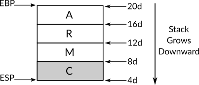
Figure 12: A New Item Pushed Into a Stack that Grows Downward
This visualization is just one way to view how the run-time stack grows, which means they may be other visualizations, and the most obvious one is to reverse the one that we just described by putting the smaller addresses on the top and the larger addresses on the bottom as shown in figure 13, you can note that in contrast to figure 12 the smallest address 4d is on top, so, based on this visualization the stack grows upward! Actually this latter visualization of run-time stack is the one which is used in Intel's manual and the term expand-up is the term that is used in the manual to describe the direction of stack growth.
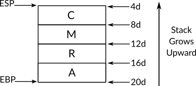
Figure 13: A Stack that Grows Upward Instead of Downward
To sum it up, the direction in which the run-time stack grows (down or up) depends on how do you visualize the run-time stack, as in figure 12 or as in figure 13. In our discussion in this book we are going to depend on the first visualization35, so, simply, the run-time stack of x86 grows downward.
2.6.5 The Problem of Resizing the Run-time Stack
We have emphasized that x86 run-time stack by default grows downward, this default behavior can be changed if we wish to, which is going to make the run-time stack to grow upwards instead and the way to do that is to use expansion-direction flag of run-time stack's segment descriptor, we have mentioned this flag when explained the structure of segment descriptor and postponed its details till here.
When we want the run-time stack to grow downward (or in Intel's term which depends on the second visualization of run-time stack: expand-up) the value of this flag should be 0, on the other hand, when we want the run-time stack to grow upward (in Intel's term: expand-down) the value of this flag should be 1. Modern operating systems use the default behavior (downward growth), we will see that this design decision is taken due to the choice of flat memory model by modern operating systems. However, the other available option (upward growth) is there to solve a potential problem and whether this problem is going to show up in a specific kernel depends on how this kernel's architecture is designed, that is, which memory model is used in this kernel.
This problem, which we can solve by making the run-time stack grows upward instead of downward, is related to the need of increasing the size of run-time stack and the fact that the run-time stack stores memory addresses 36 on it. Let's assume that our kernel created a new stack segment for a specific process X and this stack segment has a fixed size which is 50 bytes 37 for example. The process X starts its work and at some point of time its run-time stack of size 50 bytes becomes full which means that we need to resize it and make it bigger so it can hold more items, let's assume the new size will be 60 bytes.
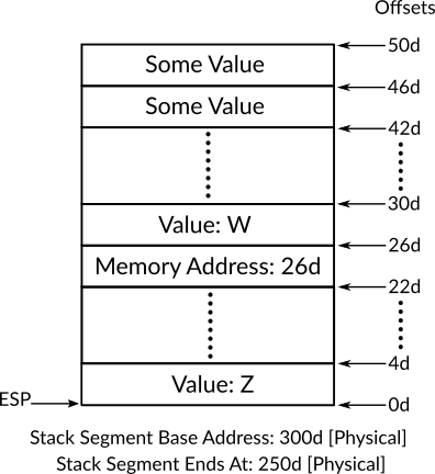
Figure 14: Process X's Run-time Stack
Before going any further with our discussion, let's see the figure 14 which represents a snapshot of process X's run-time stack when it became full. We can see from the figure that X's stack segment starts from the physical memory address 300d (segment's base address) and ends at the physical memory address 250d, also, the items of run-time stack are referred to based on their offsets inside the stack segment. We can see that a bunch of values have been pushed onto the stack, some of those values are shown on the figure and some other are omitted and replaced by dots which means that there are more values here in those locations. Normal values are called "some value" in the figure and the last pushed value in the stack is the value Z. Also, a value which represents a logical memory address has been pushed onto the stack, more accurately, this value represents an offset within the current stack segment, a full logical memory address actually consists of both offset and segment selector as we have explained earlier in this chapter when we discussed address translation. But for the sake of simplicity, we are going call this stored value as "memory address" or "memory location" in our current explanation. As we explained earlier, all memory addresses that the processes work with are logical and not physical. The value 26d is a local variable P of the type pointer (as in C) which points to another local variable R that has the value W and is stored in the memory location 26d.
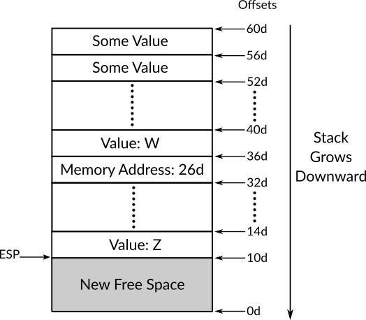
Figure 15: Process X's Run-time Stack After Resize (Grows Downward)
Figure 15 shows X's stack after resize, as you can see we have got our new free space of 10 bytes, also, because the stack grows downward so the new free space should be added on the bottom of the stack to be useful which means the previous offsets should be changed, therefore, the largest offset 50d has been updated to 60d by adding 10d (which is the newly added free space to the stack in bytes) to it and so on for the rest of offsets, also, ESP has been simply updated in the same manner.
Now we can see that the process of updating the offsets, that we are forced to perform because the stack grows downward, has caused a problem in the offsets which have been pushed onto the stack before resizing it. You can see the pointer P which still has the original value 26d, that means it doesn't point the the variable R anymore, instead it is going to point to another memory location now with a value other than W, and the same problem holds for all pushed EBP values on X's stack.
A potential solution for this problem is to update all stack items that contain memory addresses in the range of the stack after resizing it, exactly as we have done with EBP, but more simpler solution is to make the stack to grow upwards instead of downwards! Modern operating systems solves this problem by not dividing the memory into segments but they use flat memory model which views the memory as one big segment for all data, code and stacks.
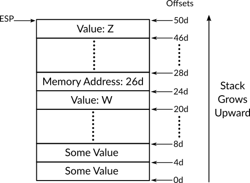
Figure 16: Process X's Run-time Stack (Grows Upward)
Now let's see what happens in the same scenario but with changing the growth direction of the stack from downward which caused the problem to upwards. In this case, as we have said before, the new items will be stored on the larger memory addresses (offsets to be more accurate). Figure 16 shows the same snapshot of X's run-time of stack as in the one of figure 14 but this time it grows upwards instead of downward. You can notice that the older values are now on the bottom of the stack, that is, on smaller memory addresses, what interests us in this stack is the entry which stores the memory address 20d that points to the memory location which has the value W and it is the one which caused the problem in the first place. When the stack was growing downward, the memory location of the value W was 26d, but this time it is 20d. So, what happens when we need to resize this run-time stack?
In the same way of the previous one, the limit of the stack (its largest offset) will be increased from 50d to 60d as shown in figure 17, but in contrast to the previous one, we don't need to update the value of ESP anymore, because as you can see from the two figures 16 and 17 the memory address 50d represents the top of the stack on both stacks. The same holds true for the stack item which stores the memory address 20d, we don't need to update it because the value W is still on the same memory address (offset) and can be pointed to by the memory address 20d. So, we can say that deciding the direction of run-time stack growth to be upward instead of downward can easily solve the problem of getting wrong stored memory address after resizing the run-time stack 38 and that's when we use segmentation as a way of viewing the memory.
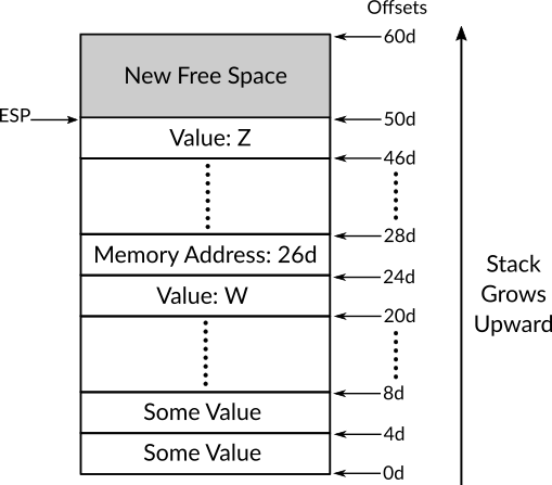
Figure 17: Process X's Run-time Stack (Grows Upward) Resized
2.7 x86 Interrupts
Event-driven programming is a common programming paradigm that is used in many areas of programming. One of these areas is graphical user interface (GUI) programming, also, it is common in game development, furthermore, some network programming frameworks use this paradigm. In this paradigm, the program is driven by events, that is, it keeps idle and waiting for any even to occur and once an event occurs the program starts to work by handling this event, for example, a mouse click is considered as an event in GUI programming. When an event occurs, the program handles this event through, usually, a separated function which is dedicated for this event, this function is known as a handler. In GUI programming for example, when the user clicks on a specific button, that is, when this event occurs, a function specified for this event on this button (the handler) is called to perform some operation after this click, such as, save a document or close the application.
This paradigm is also used by x86. When a process is running, something can interrupt (an event occurred) the processor which is going, in this case, to stop the execution of the current process temporarily, and call the suitable interrupt handler (also called interrupt service routine) to handle the current interrupt, after handling the interrupt, the processor can resume the process which was running before the interrupt occurred.
One example of the usage of interrupts in this low-level environment is the system timer. In the hardware level, there could be a system timer which interrupts the processor in each X period of time and this type of interrupt is the one that makes multitasking possible in uniprocessor systems. When a processor is interrupted by the system timer, it can call the kernel which can change the currently running process to another one; this operation known as scheduling which its goal is distributing the time of the processor to the multiple processes in the system.
Another example of using interrupts is when the user of an operating system presses some keys on the keyboard, these events of pressing keyboard keys should be sent to the kernel which is going to delegate the device driver 39 of the keyboard to handle these events in a proper way, in this case, with each key press, the keyboard is going to interrupt the processor and request to handle these events.
In x86, both hardware and software can interrupt the processor, system timer and keyboard are examples of hardware interrupts while the software interrupt can occur by using the x86 instruction int which we have used when we wrote our bootloader, the operand of this instruction is the interrupt number, for example, in our bootloader we have used the following line int 10h, in this case, the interrupt number is 10h (16d) and when the processor is interrupted by this instruction, it is going to call the handler of interrupt number 10h. Software interrupt can be used to implement what is known as system calls which provide a way for user applications to call a specific kernel's code that gives the applications some important services such as manipulating the filesystem (e.g. reading or writing files, create new file or directories, etc.) or creating new process and so on in a way that resembles the one that we used to call BIOS services.
In addition to interrupts, exceptions can be considered as another type of events which also stop the processor from its current job temporarily and make it handle it and then resume its job after that. The main difference between exceptions and interrupts in x86 is that the former occurs when an error happens in the environment, for example, when some code tries to divide some number by zero, an exception will be generated and some handler should do something about it, we can perceive the exceptions of x86 as the exceptions of some programming languages such as C++ and Java.
2.7.1 Interrupt Descriptor Table
In x86, there is a table known as interrupt descriptor table (IDT), also may called interrupt vector table but the term that Intel uses is the former one while the latter are used to describe this kind of tables as a concept in some works of literature and not the name of the table on a specific architecture. IDT resides in the memory and tells the processor how to reach to the handler of a given interrupt number. The entries of IDT are known as gate descriptors and the size of each one of them is 8 bytes same as GDT and LDT. At most, IDT can contain 256 gate descriptors and the base memory address of IDT is stored in a special register known as IDTR.
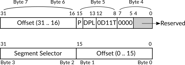
Figure 18: Gate Descriptor Structure for Interrupt and Trap Gates
The gate descriptors in the IDT table can be of three types, task gate, interrupt gate and trap gate, our focus currently will be on the latter two. The structure of both interrupt and trap gate descriptor is shown in figure 18. As we have said earlier, a gate descriptor of the IDT should point to the memory address of the interrupt handler's code. We can see in the figure that bytes 2 and 3 should contain a segment selector, which is the segment selector of handler's code, that is, the index of the code segment that contains handler's code, we can see an important difference between GDT and IDT here. In the former the base address of a segment is a linear address, while the base address of the handler is a logical address.
The offset of the first handler's instruction should be set in the descriptor, this will be useful if the handler's code is just a part of the whole code segment which is presented in the segment selector field. The offset in the gate descriptor is divided into two parts, the least significant2 bytes of the offset should be loaded into bytes 0 and 1 of the descriptor, while the most significant2 bytes of the offset should be loaded into bytes 6 and 7.
The least significant nibble of byte 4 is reserved and the most significant nibble of byte 4 should always be 0d. The most significant bit of byte 5 is present flag (P flag), when its value is 0 that means the code that this descriptor is pointing to is not loaded into memory, while the value 1 means otherwise. The descriptor privilege level field (DPL) contains the privilege level of the handler, it occupies the second and third least significant bit of byte 5. The value of fourth, sixth and seventh least significant bits of byte 5 should always be 0b, 1b and 1b respectively. The flag which is called D in the figure specifies the size of the gate descriptor itself whether it is 32 bits, whenD flag = 1, or 16 bits when D flag = 0, the former should always be our choice in protected-mode, while the latter should always be our choice in real-mode. The flag which is called T in the figure specifies whether the gate is an interrupt gate, when T flag = 0, or the gate is an trap gate, when T flag = 1.
The difference between interrupt and trap gates is too simple, when a handler defined as an interrupt gate is called, the processor is going to disable the ability to signal a new interrupt until the handler returns, that is, the execution of the handler will not interrupted until it finishes its job and return to the caller, of course there are some exceptions, a type of interrupts known as non-maskable interrupts (NMI) will interrupt the execution of the current code even if the interruption is disabled, non-maskable interrupts occur when some catastrophic event (from the hardware perspective) happens in the system. On the other hand, the handler that is defined as a trap gate can be interrupted by any new interrupt, that is, the interruption will not be disabled by the processor.
However, disabling interruption is an operation that can be performed by the code by using the x86 instruction cli (still, non-maskable interrupts are excepted) which stands for clear interrupt flag and can be enabled again by using the instruction sti which stands for set interrupt flag, both of these instructions manipulate the value of interrupt flag which is a part of the register EFLAGS.
Now, let's assume that we have defined a gate descriptor for a handler, let's name it A. The question is, which interrupt the handler A is going to handle? In other words, for which interrupt number the processor is going to call the code of A to handle the interrupt? In fact, that depends on the index of A's gate descriptor in the IDT table. Let's assume that the index is 0d, then A's code will be called when the interrupt number 0 is signaled, that means the term interrupt number is a synonym for entry's index number in IDT table
In protected-mode, interrupt numbers, that is IDT entries indices, from 0 to 21 have specific meaning defined by x86 architecture itself, for example, the interrupt number that is reserved for division by zero exception is the interrupt number 0 and, in our example, the code of A will be called when some other code divides a number by zero. Beside interrupt numbers 0 to 21, the range of interrupts number from 22 to 31 are reserved, and the interrupt numbers from 32 to 255 are available for the system programmer to decide their meanings, however, not all of their descriptors should be filled, only the needed ones will be enough.
2.7.1.1 The Register IDTR
In same way as GDT, we should tell the processor where the IDT reside in the memory and that can be performed by the instruction lidt which stands for load IDT, this instructions works as lgdt, it takes an operand and loads it to the register IDTR which will be used later by the processor to reach to the IDT table.
The structure of IDTR is same as GDTR, its size is 48 bits and it's divided into two parts, the first part represents the size of the IDT in bytes, that is, the IDT's limit, this field starts from bit 0 of IDTR and ends at bit 15. Starting from bit 16 up to bit 47 the base linear address 40 where IDT is reside should be set.
If some of these terms are new for you don't worry about them too much, you will learn them gradually throughout this book.↩
That is, the user of the operating system can only run one process at a given time. DOS is a an example of monotasking operating system.↩
Segmentation will be examined in details later on this chapter.↩
That is, the processes which runs on privilege level greater than
0↩For example, loading
GDTregister by using the instructionlgdtas we will see later in this chapter.↩And from here came the well-known joke: "There are 10 types of people in this world, those who understand binary and those who don't".↩
I think It's too brave to state this claim, however, it holds true at least for the well-known numbering system.↩
Can you tell why? [Hint: How the maximum hexadecimal number
Fis represented in binary?]↩The architecture which each memory address points to
1 byteis known as byte-addressable architecture or byte machines. It is the most common architecture. Of course, other architectures are possible, such as word-addressable architecture or word machines.↩The concept and term of offset is not exclusive to segmentation, it is used on other topics related to the memory.↩
Yes, all segments can be on the same memory location, that is, there is a
64KBsegment of memory which is considered as the currently active code segment, data segment and stack segment. We have already mentioned that when we have discussed how to implement flat-memory model on x86.↩Which loads the physical memory address of
title_stringto the registersi.↩This is a relaxed definition of segment selector, a more accurate one will be presented later.↩
In real mode, the starting address of the segment is stored directly on the corresponding segment register (e.g.
CSfor code segment).↩Reminder: In protected mode, the corresponding segment register stores the selector of the currently active segment.↩
And it should, since segmentation is enabled by default in x86 and cannot be disabled.↩
Remember our discussion of the difference between our logical view of the memory (e.g. segmentation) and the actual physical hardware↩
We can see here how obvious the mapping between the logical view of the memory and the real-world memory.↩
Don't worry about paging right now. It will be discussed later in this book. All you need to know now is that paging is another logical view of the memory. Paging is disabled by default in x86 which makes it an optional feature unlike segmentation.↩
Which means do enable read, since
1is equivalent totruein the context of flags.↩Which means don't enable read.↩
Which makes sense, enabling reads from a code segment means it contains data also.↩
We use the term access here for both types of application segments. While this term is valid for data segment, we mean execute for code segment.↩
The processor knows it is a stack segment if the segment selector is loaded into stack segment selector register
SS↩In terms of Intel's manual: compatibility mode.↩
More accurately, the linear address. Refer to discussion of memory translation process in this chapter.↩
More accurate definition of a segment selector and its structure in protected-mode is presented in the next subsection.↩
On contrary, queue data structure stores data in first-in-first-out (FIFO) manner.↩
That doesn't mean no more operations can be defined for a given data structure in the implementation level. It only means that the conceptual perspective for a given data structure defines those basic operations which reflect the spirit of that data structure. Remember that when we start to use x86 run-time stack with more operations than
pushandpoplater, though those other operations are not canonical to the stack data structure, but they can be available if the use case requires that (and yes they may violate the spirit of the given data structure! We will see that later).↩Which is implemented by default in most major programming languages and know as arrays (in C for example) or lists (as in Python)↩
Some programming languages, especially those which are derived from Algol differentiate between a function which should return a value to the caller, and a procedure which shouldn't return a value to the caller.↩
We claim that for the purpose of explanation. But actually the matter of separated run-time stack for each process is a design decision that the operating system's kernel programmer/designer is responsible for.↩
In fact, x86 is little-endian architecture which means that
0x10will be stored in the location100dwhile0x04will be stored in the location101dbut I've kept the example in the main text as is for the sake of simplicity.↩As a reminder, don't forget that all these memory address are actually offsets inside a stack segment and not a whole memory address.↩
And many other books actually uses the first visualization as I recall and for that I chose it in this book. And according to my best knowledge the only reference that I've seen that depends on the second visualization is Intel's manual.↩
The previous values of
EBPandEIP. Also the application programmer may store memory addresses of local variables in the stack (e.g. by using pointers in C).↩As you may recall, the size of the segment can be decided by the base address of the segment and its limit as specified in the segment's descriptor.↩
Actually, the well-know stack overflow vulnerability in x86 is also caused by stack growing downward and can be avoided easily in growing upwards stacks!↩
That's why in some kernel's designs, especially, monolithic kernel keeps the device drivers as a part of the kernel.↩
As we have mentioned multiple time that in our current case, where the paging is disabled, a linear address is same as physical address.↩